User Material Models
Introduction
IMPETUS Solver comes with support for user defined material models. Our solution is to let the user compile a DLL (dynamic-link library) file which then is linked to the solver during the start of a simulation. The user material is not compiled into the software itself and it allows for several advantages. Since object code of the software isn't needed, it will works with any version of the solver (unless we've done major changes to the interface). This means one can use the latest version of the Solver. We allows up to five different user defined material models.
Structure
The user material zip file (provided by our support) contains a Visual Studio 2022 solution with two project folders inside. The C++ project "mat_user_functions" contains a wrapper to call built-in subroutines/functions from the solver. Do not edit the files inside this project. The other project "mat_user" which is an Intel Fortran project, contains the code for user defined material models. There are several files inside this project: mat_user.F, a few mat_XXXX.F files (examples) and custom_functions.F. As the name suggests, custom_functions.F can be used to define custom subroutines/functions. This is completely optional but we recommend using it. The file mat_user.F is the main file and this is the one that should be modified. Start by opening mat_user.sln with Visual Studio. Before compilation, remember to change compilation mode from Debug to Release.
Now, expand "mat_user" project from the solution tree and open mat_user.F under "Source Files". We've provided with some example models which are implemented in different files, but called by mat_user_1(), mat_user_2(), mat_user_3() and mat_user_4(). Feel free to modify these and customise them to your needs. The example in mat_user_1() is similar to our built-in *MAT_METAL material model.
After the compilation, mat_user.dll will be copied to the output folder located in the root directory of the Visual Studio project. When executing a simulation, check the "Use defined material model" checkbox and add the path to the file.
Following subroutines are defined in the mat_user.F file:
- mat_user_X(): Main subroutine for the user material X (X: 1-5)
- init_mat_user_X(): Initialisation subroutine for the user material X (X: 1-5)
- mat_user_set_state_variables(): Set the number of state variables, state variable output, texture location (for fibre directions) and damage type location
Arguments for mat_user_X():
| Argument | Description |
|---|---|
| strain(6) | Total strain tensor |
| dstrain(6) | Strain increment tensor |
| stress(6) | Stress tensor |
| F(9) | Deformation gradient |
| U(6) | Right stretch tensor |
| ifail | integer variable to set if the current integration point has failed or not |
| iface_update | Integer variable to force update of faces |
| hist(*) | History state variable array (Size defined in mat_user_set_state_variables()) |
| cmat(100) | Material parameters |
| stiffness(4) | Used for time step calculation. 1 = shear, 2 = bulk, 3 = xi, 4 = bfac |
| iel | Element ID |
| ip | Integration point ID (local ID for the specific element) |
| itype | Element type |
| dt1 | Current time step size |
| tt | Current time |
Arguments for init_mat_user_X():
| Argument | Description |
|---|---|
| hist(*) | History state variable array. Size defined in mat_user_set_state_variables() |
| cmat(100) | Material parameters |
| stress(6) | Stress tensor |
| strain(6) | Strain tensor |
| stiffness(4) | Used for time step calculation. 1 = shear, 2 = bulk, 3 = xi, 4 = bfac |
| x | Node coordinate |
| iel | Element ID |
| ip | Integration point ID (local ID for the specific element) |
| itype | Element type |
Getting started
Symmetric tensors
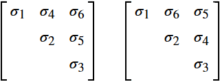
All symmetric tensors in our solver uses an alternative notation of the Voigt notation. The traditional voigt notation for a 3X3 matrix is defined as: 11, 22, 33, 23, 13, 12. Our definition is: 11, 22, 33, 12, 23, 13.
Material parameters
Material parameters defined in the *MAT_USER_X command can be accessed by the cmat array. Position 1-6 are tied to the first row after the material ID definition (1st value). For example cmat(1) tied to the 2nd value, cmat(2) the 3rd, cmat(3) the 4th, etc. For a normal use case, we use the following: cmat(1) = density, cmat(2) = young's modulus, cmat(3) = poisson's ratio, etc.
Second row starts at index cmat(7), third row at cmat(15), forth row at cmat(23), etc.
There are a few slots in cmat which are reserved. cmat(43) and cmat(44) are reserved for pre-calculated shear and bulk modulus. cmat(80) and cmat(81) are used for damage and erosion.
Example:
! material data from input: density, young's modulus and poisson's ratio

! *MAT_USER_1
! 1, 7800.0, 2.0e9, 0.3

dens        = cmat(1) ! 7800.0
young       = cmat(2) ! 2.0e9
pr          = cmat(3) ! 0.3

! pre-calculated
shear       = cmat(43)
bulk        = cmat(44)

! these variables are automatically set depending damage and erosion type
damage_type = nint(cmat(80))
erode_flg   = nint(cmat(81))
State variables
The state variable array is a container where one can store data for each integration point. These variables can change throughout the simulation. Examples of typical variables are "Effective Plastic Strain" and "Damage". To use state variables, use the hist array to load and store data. It's a good idea to set initial values for these variables in init_mat_user_X() subroutine.
Example of loading and storing state variables:
! load state variables: effective plastic strain, damage and yield stress
epsp  = hist(1)
dmg   = hist(2)
sigy0 = hist(3)

! some code involving epsp, dmg and/or sigy0
[...]

! save state variables
hist(1) = epsp
hist(2) = dmg
hist(3) = sigy0
Before state variables can be used, one needs to define the size of the array. This is done by editing mat_user_set_state_variables() in mat_user.F. In our examples, these are set in the subsequential subroutine calls since they are implemented in different files). For example, see mat_template_state_variables() in mat_template.F (which is called by mat_user_set_state_variables() in mat_user.F).
For instance, if we are going to specify the number of history variables for mat_user_1(), we need to assign a value to num_variable(1). In the example (see code below), we have set the size to 3 for position 1 in the num_variable() array. Position 1 indicates user material ID 1, value 3 is the number of state variables for this user material.
num_variable(1) = 3
State variables as contour plot
With the size set, we are ready to go but we will not be able to plot these values in the GUI. None of these values are written to our output files by default. To add a state variable to the output, we need to tell the solver to output it. This can be done by calling mat_user_set_name(). variable_id tells which index in the state variable array to output. variable_name specifies the name the state variable should have.
user_material_id         = 1
variable_id              = 1
variable_name(1:40)      = "Effective plastic strain"
call mat_user_set_name(user_material_id, variable_id, variable_name)

variable_id              = 2
variable_name(1:40)      = "Damage"
call mat_user_set_name(user_material_id, variable_id, variable_name)
They can be found under the "General" category in Contour plot. The prefix "User: " will automatically be added to the name when using Contour plot in the GUI.
Curves & functions
Curves & functions can be used in the user material models just like in *MAT_METAL. To use curves, one needs to tell the solver where in the material parameter list the curve is located. This can be done by editing mat_user_set_state_variables() and modify/add the array user_curve_location. This is a 2D array with two arguments defining user curve ID and material ID. For instance, if we have two curves and want both defined, we simply add:
user_curve_location(1, 1) = 7
user_curve_location(2, 1) = 8
This will tell the solver that there are curves in positions 7 and 8 in the material parameter array (cmat) for mat_user_1. Position 7 and 8 represents the two first columns on the second line in the *MAT_USER_X command. More information about how to call curves and functions can be found in the section "Built-in subroutines/functions" further down in this document.
Texture location
When implementing material models using fibre direction (for example fibre composites) with *INITIAL_MATERIAL_DIRECTION_WRAP, a texture location must be set. The location tells IMPETUS Solver where in the state variables array (hist) to set the initial fibre direction. It requires 9 slots (3 vectors) in the state variables array (from the specified index) so make sure to allocate enough space when setting num_variable().
Example below shows allocation of 14 state variables and that we set the last 9 of them for initial fibre direction:
num_variable(1)     = 14
texture_location(1) = 6
Damage definition
Material failure can be defined as element erosion or node splitting. The variable damage_location defines where in the state variable array that damage is located. This variable is only needed for node splitting but we recommend to set it anyway even when not using node splitting. erode_flg defines if the material model should use element erosion (=1), node splitting (=2) or none (=0). If erode_flg_pos is set, the value of the material parameter (cmat) in that specified location will determine to use element erosion or node splitting.
damage_location          = 2
erode_flg                = 2
erode_flg_pos            = 0
call mat_user_set_damage(user_material_id, damage_location, erode_flg, erode_flg_pos)
This should enough for node splitting since the Solver will handle the rest. For element erosion, failure handling must be defined manually. To do this, add this after the damage calculations in mat_user_X():
! element erosion (node splitting will not execute this if-statement)
if (dmg.ge.1.0d0.and.erode_flg.lt.2) then
  dmg = 1.0d0

! reset deviatoric stresses
  stress(:) = 0.0d0

! erosion -> set failure flag
  if (erode_flg.eq.1) ifail = ifail + 1
endif
We set the dmg variable to 1.0, reset the stress array and we increment ifail with 1. If enough integration points per element fails, then the solver will automatically erode it. This code can co-exist with node splitting capability since node splitting will set the erode_flg variable to 2. If that happens then this code will never be executed.
Built-in subroutines/functions
We've made some of the core functionality of the solver available. Return values from the subroutines are marked with underscore in the parameter list. Functions return its value as return values.
Load Curve / Function
The last 5 parameters (p, epsp, sigy0, T & dmg) are for functions. They must be set to 0 if not being used. This call can be used both to call curves and functions.
| Parameter | Description |
|---|---|
| idlc | Function/Curve ID (integer) |
| x | Value of x in function f(x) (double precision) |
| f | Return value (double precision) |
| p | Pressure parameter (double precision) |
| epsp | Old effective plastic strain parameter (double precision) |
| sigy0 | Yield stress parameter (double precision) |
| T | Thermal parameter (double precision) |
| dmg | Damage parameter (double precision) |
! Load a curve
call load_curve(idlc, epsp+deps, sigy1, 0, 0, 0, 0, 0)

! Load a curve or a function with pressure and effective strain rate variables set
call load_curve(idlc, epsp+deps, sigy1, p, epsp, 0, 0, 0)

! Load a curve or a function width all parameters set
call load_curve(idlc, epsp+deps, sigy1, p, epsp, sigy0, T, dmg)
Normalise a vector
This subroutine will return normalised v and also its length x.
| Parameter | Description |
|---|---|
| v | 3-component vector (double precision) |
| x | length (double precision) |
Cross product
This subroutine will return the cross product between a1 & a2 in a3.
| Parameter | Description |
|---|---|
| a1 | 3-component vector (double precision) |
| a2 | 3-component vector (double precision) |
| a3 | Return value, 3-component vector (double precision) |
Dot product
Returns the dot product between v1 and v2.
| Parameter | Description |
|---|---|
| v1 | 3-component vector (double precision) |
| v2 | 3-component vector (double precision) |
Polar decomposition
This subroutine computes the polar decomposition and returns new values for R, U & Uinv.
| Parameter | Description |
|---|---|
| F | Positive definite tensor (3X3) (double precision) |
| R | Rotation tensor (3X3) (double precision) |
| U | Symmetric stretch tensor U (double precision) |
| Uinv | Inverted symmetric stretch tensor (double precision) |
Eigenvalues of symmetric 3X3-matrix
This subroutine returns the eigen values calculated from avec.
| Parameter | Description |
|---|---|
| avec | 6-component tensor (double precision) |
| eigval | Returns 3-component vector (double precision) |
Eigenvectors of symmetric 3X3-matrix
This subroutine returns the eigen values calculated from avec.
| Parameter | Description |
|---|---|
| avec | 6-component tensor (double precision) |
| eigval | 3-component vector (double precision) |
| eigvec | Returns two eigenvectors eigvec(1) and eigvec(4) in one 6-component array (double precision) |
! First, find eigenvalues and then use them to find the eigenvectors
 call eigval_3x3_symm(stress, eigval)
 call eigvec_3x3_symm(stress, eigval, eigvec)
Invert 3X3-matrix
This subroutine returns the eigen values calculated from avec.
| Parameter | Description |
|---|---|
| A | 3X3 matrix to be inverted (double precision) |
| B | Return value, inverted matrix (double precision) |
| detA | Return value, determinant (double precision) |
Volume of an element
Returns volume of an element in double precision.
| Parameter | Description |
|---|---|
| iel | Element ID (integer) |
| itype | Element type (integer) |
Volume of an integration point
Returns volume of an integration point in double precision.
| Parameter | Description |
|---|---|
| iel | Element ID (integer) |
| itype | Element type (integer) |
| ip | Integration point ID (integer) |
Initial volume of an integration point
Returns initial volume of an integration point in double precision.
| Parameter | Description |
|---|---|
| iel | Element ID (integer) |
| itype | Element type (integer) |
| ip | Integration point ID (integer) |
Get element nodes
This subroutine returns an array of node IDs of a specific element.
| Parameter | Description |
|---|---|
| iel | Element ID (integer) |
| itype | Element type (integer) |
| n | Return value, array (integer) |
Get element neighbors
This subroutine returns an 2D array of neighboring elements and the number of neighbors. First value of the array contains the neighboring element ID. The second value contains the element type of the neighboring element.
| Parameter | Description |
|---|---|
| iel | Element ID (integer) |
| itype | Element type (integer) |
| list | Return value, 2D array (integer) |
| num_neigh | Return value, number of neighbors (integer) |
Get integration point coordinate
This subroutine returns the coordinate of an integration point.
| Parameter | Description |
|---|---|
| iel | Element ID (integer) |
| itype | Element type (integer) |
| ip | Integration point (integer) |
| xip | Return value, 3-component vector (double precision) |
Element conversion (internal to user ID)
Returns user (external) ID of an element.
| Parameter | Description |
|---|---|
| iel | Element ID (integer) |
| itype | Element type (integer) |