COORDINATE_SYSTEM

Coordinate system
*COORDINATE_SYSTEM
"Optional title"
csysid, $x_0$, $y_0$, $z_0$, pid, curve
$\hat{x}_x$, $\hat{x}_y$, $\hat{x}_z$, $\bar{y}_x$, $\bar{y}_y$, $\bar{y}_z$
Parameter definition
VariableDescription
csysid Unique identification number
$x_0$, $y_0$, $z_0$ Initial coordinate of origin
pid Optional part ID
default: not used
curve Flag to activate generation of CURVE files
options:
0 $\rightarrow$ curve file output inactive
1 $\rightarrow$ curve file output active
$\hat{x}_x$, $\hat{x}_y$, $\hat{x}_z$ Initial direction of local x-axis
$\bar{y}_x$, $\bar{y}_y$, $\bar{y}_z$ Vector needed for the definition of the local y- and z-axis
Description

This command defines a local cartesian coordinate system. The system is forced to follow the translation and rotation of the finite element in which it is embedded at time 0 (Lagrangian description of motion). Hence, the origin of the system must be located on the surface of, or embedded inside, the finite element mesh.

The origin is initially located at ($x_0$, $y_0$, $z_0$) and the local x-direction is ($\hat{x}_x$, $\hat{x}_y$, $\hat{x}_z$). The local z-direction is defined as $\hat{\mathbf{z}} = \hat{\mathbf{x}} \times \bar{\mathbf{y}} / \vert \hat{\mathbf{x}} \times \bar{\mathbf{y}} \vert$ and the local y-direction as $\hat{\mathbf{y}} = \hat{\mathbf{z}} \times \hat{\mathbf{x}}$.

The part ID (pid) is only needed when the initial location of the origin is right in the boundary between two different parts and when the system needs to be tied to one of these parts.

Setting curve=1 instructs Impetus Solver to generate CURVE files containing the coordinate system velocity and spin as functions of time. The purpose of this feature is to document displacements and rotations at specific points in large models, in a format that easily can be re-used as input to other models. A typical application is sub-modeling, wherein local displacements in a global model serve as boundary conditions for smaller, more detailed sub-models.

The generated velocity and spin curves are named:

csys_curve_vx_X.k (X = coordinate system ID)
csys_curve_vy_X.k
csys_curve_vz_X.k
csys_curve_ohmx_X.k
csys_curve_ohmy_X.k
csys_curve_ohmz_X.k

Note that, for fixed (Eulerian) coordinate systems, there is a special command COORDINATE_SYSTEM_FIXED.

Example
Coordinate system and a fixed coordinate system

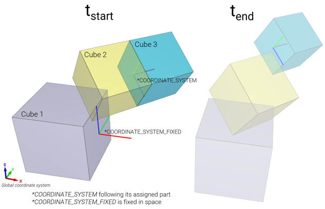
A simple model demonstrating differences between COORDINATE_SYSTEM and COORDINATE_SYSTEM_FIXED.

Cube 1 is created with a fixed coordinate system while the other cubes are created with a tilted coordinate system with its origin located on the boundary between them. The coordinate system is given an optional part ID of 3 which ties it to cube 3. The cubes are set in motion and as cube 3 separates from cube 2, the coordinate system is forced to follow cube 3 while the fixed coordinate system remains at its initial location.


*UNIT_SYSTEM
SI
*PARAMETER
%tend = 0.01, "Termination time"
%disp_x = 2, "Displacement in X of cube"
%disp_y = 2, "Displacement in Y of cube"
%L = 1, "Side length cube"
#
# --- TIME and OUTPUT ---
#
*TIME
[%tend], , , 1e-4
*OUTPUT
[%tend/5]
#
# --- MESH ---
#
*COMPONENT_BOX
1, 1, 2, 2, 2, 1
[-%L], [-%L/2], [-%L/2], 0, [%L/2], [%L/2]
*COMPONENT_BOX
2, 2, 2, 2, 2, 2
[-%L], [-%L/2], [-%L/2], 0, [%L/2], [%L/2]
*COMPONENT_BOX
3, 3, 2, 2, 2, 2
0, [-%L/2], [-%L/2], [%L], [%L/2], [%L/2]
#
# --- MATERIAL ---
#
*MAT_RIGID
1, 7800
*PART
1, 1
2, 1
3, 1
#
# --- COORDINATE SYSTEMS ---
#
*COORDINATE_SYSTEM_FIXED
1, 1, 0.5, 0.5
*COORDINATE_SYSTEM
2, 1, 2.5, 0.5, 3
cos(45), sin(45), 0, 2, 1, 1
#
# --- MOTION IN GLOBAL X-DIRECTION ---
#
*BC_MOTION
"All cubes"
1
ALL
D, X, 1
*FUNCTION
1
smooth_d(%disp_x, 0, %tend)
#
# --- MOTION IN GLOBAL Y-DIRECTION (CUBE 3) ---
#
*BC_MOTION
"Cube 3"
4
P, 3
D, Y, 2
*FUNCTION
2
smooth_d(%disp_y, 0, %tend)
*END
Sub-model using curve data

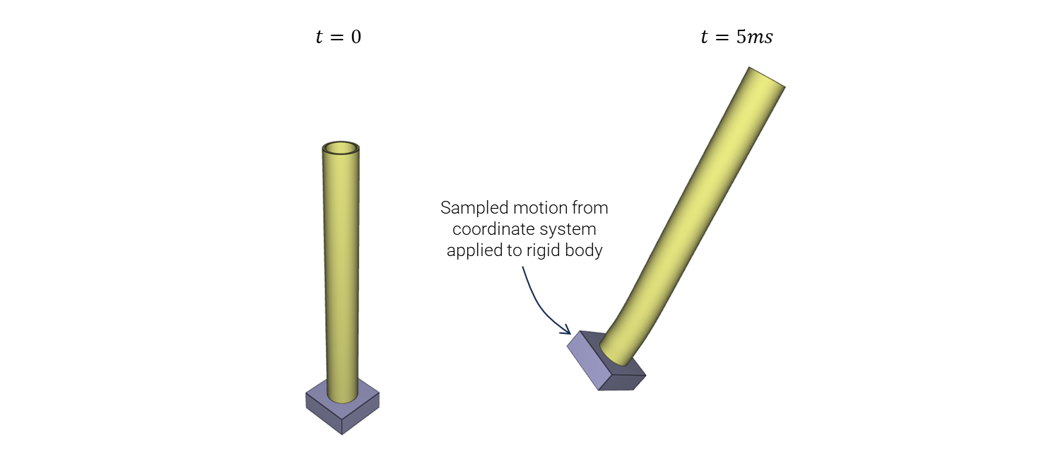
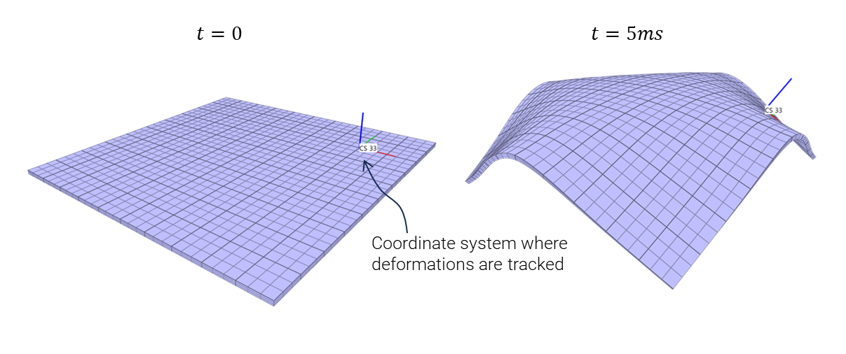
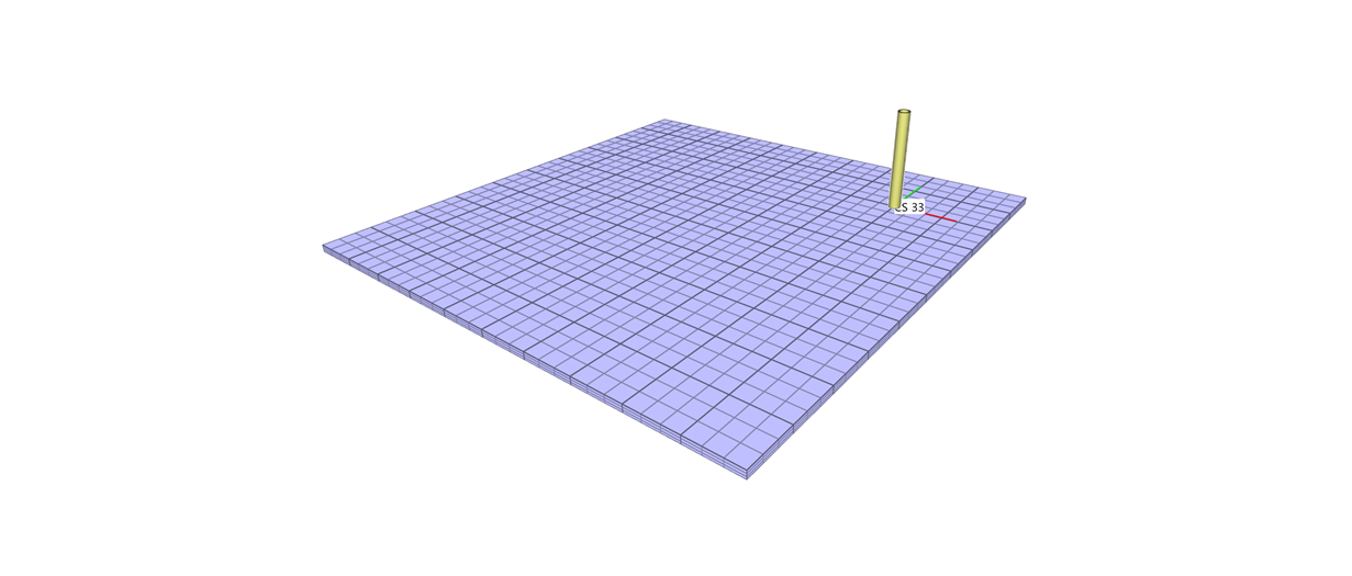
In this example a steel plate is exposed to an initial velocity field. A coordinate system is attached to a point on the plate surface. The coordinate system represents the location of a sub-structure, in this case an aluminium pipe. Using the option curve=1 the coordinate system velocity and spin histories are written to local files as CURVE commands.

Plate with attached coordinate system
Plate with imagined location of pipe
#
# STEP 1: Deforming steel plate
#
*UNIT_SYSTEM
SI
#
# --- TIME ---
#
*TIME
0.005
#
# --- MESH ---
#
*COMPONENT_BOX
"Plate"
1, 1, 10, 10, 1
-0.5, -0.5, 0, 0.5, 0.5, 0.015
*CHANGE_P-ORDER
P, 1, 3
#
# --- MATERIAL ---
#
*MAT_METAL
1, 7800.0, 210.0e9, 0.3
1
*FUNCTION
1
6.0e8 + 6.0e8*epsp^0.3
#
# --- PART ---
#
*PART
"Plate"
1, 1
#
# --- VELOCITY ---
#
*INITIAL_VELOCITY
P, 1, 0, 0, fcn(22)
*FUNCTION
"vz"
22
100 * (1 - 4*(x^2 + y^2))
#
# --- COORDINATE SYSTEM ---
#
*COORDINATE_SYSTEM
33, 0.3, 0.3, 0.015, 1, 1
*END

In a second simulation, the generated curves are used as velocity and spin boundary conditions for the aluminium pipe. It can then be simulated alone, without having the steel plate included.

Sub-model of aluminium pipe
#
# STEP 2: Aluminium pipe
#
*UNIT_SYSTEM
SI
#
# --- CURVES FROM STEP 1 (IDs 101 to 106) ---
#
*INCLUDE
csys_curve_vx_33.k
*INCLUDE
csys_curve_vy_33.k
*INCLUDE
csys_curve_vz_33.k
*INCLUDE
csys_curve_ohmx_33.k
*INCLUDE
csys_curve_ohmy_33.k
*INCLUDE
csys_curve_ohmz_33.k
#
# --- TIME ---
#
*TIME
0.005
#
# --- MESH ---
#
*COMPONENT_BOX
"Base"
1, 1, 1, 1, 1
0.28, 0.28, 0, 0.32, 0.32, 0.015
*COMPONENT_PIPE
"Pipe"
2, 2, 20, 12, 1
0.3, 0.3, 0.015, 0.3, 0.3, 0.215, 0.01, 0.012
*CHANGE_P-ORDER
P, 2, 3
*SMOOTH_MESH
P, 2, 45.0
#
# --- MATERIAL ---
#
*MAT_RIGID
1, 7800.0
*MAT_METAL
2, 2700.0, 70.0e9, 0.3
2
*FUNCTION
2
150.0e6 + 200.0e6 * (1 - exp(-5*epsp))
#
# --- PART ---
#
*PART
"Base"
1, 1
"Pipe"
2, 2
#
# --- MERGE ---
#
*MERGE
"Pipe to Base"
P, 2, P, 1
#
# --- MOTION FROM STEP 1 ---
#
*BC_MOTION
"Base"
1
P, 1
V, X, 101
V, Y, 102
V, Z, 103
V, RX, 104
V, RY, 105
V, RZ, 106
*END